

Descriptive statistics
Before empirical analysis, descriptive statistics of the variables are needed. Table 2 shows the descriptive statistics of the variables mentioned in Section 3.1, including the mean value, variance, maximum value, quantiles, etc.
On the basis of the existing income data of rural residents, this study further selected the income of rural residents in 2007 and 2022 and divided it into four intervals according to its maximum value, which were depicted on the county map of China by using the mapping function of R software (Fig. 1), to explore the temporal and spatial characteristics.
Figure 2 illustrates the spatiotemporal evolution of rural income. The upper half of describes the spatial distribution characteristics of rural income in 2007 and 2022. To avoid the visual impact of excessive data points, this study used R software to calculate the average rural income (lnRIncome) at the county level for each province, rank the data, and plot it on a polar histogram. Comparing the spatial distribution of rural income between 2007 and 2022, it can be observed that in 2007, income differences among provinces were relatively small, with a more concentrated distribution. However, by 2022, income differences among provinces had significantly increased, and some provinces that previously had lower rural incomes had moved into the leading positions by 2022, such as HEB and JX. The lower left part of Fig. 2 depicts the change in residents’ income over time in ecological functional areas and non-ecological functional areas. The income growth rate of residents in ecological functional areas is significantly greater than that of residents in non-ecological functional areas. The lower right part of Fig. 2 describes the percentage accumulation of variables and the change trend over time. The proportion of residents’ income gradually increased over time. In addition to the explained variables, this study further explores the trend of control variables over time. Figure 2 shows that urbanization and air pollution have decreased annually, whereas other control variables, such as economic development and scientific and technological innovation, have increased annually. The establishment of ecological functional zones has improved the local ecological environment, reduced air pollution, promoted the development of tourism and other service industries, improved rural productivity, and narrowed the urban‒rural income gap (Yao and Jiang, 2021).

The spatiotemporal evolution of rural incomes.
Notes: The capital letter combinations in the upper half of Fig. 2 correspond to the initials of Chinese provinces, such as BJ for Beijing.
Baseline regression results
By constructing a multiperiod DID model, this study empirically tested whether key national ecological functional zones could increase rural residents’ income. The empirical results show that the implementation of ecological function regional policy significantly promotes the improvement of rural residents’ income. Table 3 shows the baseline regression results. Column 1 controlled for the county fixed effect, column 2 further controlled for the time fixed effect on the basis of column 1, and the core explanatory variable was significantly positive at the 1% level, indicating that the China’s key ecological functional areas significantly promoted the development of rural residents’ income. To account for potential missing variable bias, columns 3 and 4 add control variables further to columns 1 and 2. Column 5 further controls for province×year fixed effects on the basis of columns 3 and 4. The core explanatory variables of Column 3, column 4 and column 5, DID, were all positive and significant at the 1% level, which once again explained the promoting effect of key national ecological functional zones on rural residents’ income. Therefore, Hypothesis 1 is true.
Further observation shows that the control variables also have a significant effect on rural residents’ income. For example, the coefficient of economic development in Column 4 is 0.2821 and is positively significant at the 1% level, indicating that economic development has significantly increased rural residents’ income. In columns 3 and 4, the impact of scientific and technological innovation on rural per capita disposable income is significantly positive, possibly because technological innovation reduces unemployment and increases rural residents’ income by upgrading technology (Adriana and Wildayana, 2019).
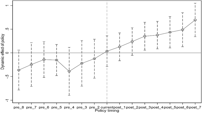
Parallel trend test
The DID model is based on the assumption that the parallel time trend is satisfied; that is, there is no significant difference in the development trend of the relevant variables of the control group and the treatment before the policy impact. Figure 3 shows the results of the parallel trend test for Model (2), showing the regression coefficient and its 95% confidence interval. As shown in the Fig. 3, before the policy, the 95% confidence interval of the time dummy variable coefficient relative to the policy had intersection points with the 0 line, there was no significant difference from 0, and there was no obvious linear trend. The test results revealed that the experimental group and the control group followed the parallel trend hypothesis. From the perspective of the dynamic effect, after the implementation of key national ecological functional zones, the dynamic effect gradually increased. The results show that the implementation of the national key ecological functional zone policy has a positive effect on increasing rural residents’ income. This result strengthens the credibility of the baseline regression results in this study. Further observation revealed that the positive impact of the key ecological functional zone policy only started to manifest in the third year postimplementation. In the initial two years, there were positive effects, but they were not statistically significant. Considering the ecological restoration cycle, the construction of ecological functional zones involves both the protection and restoration of the ecological environment, processes that may require considerable time to yield noticeable results. Consequently, it is challenging to translate these efforts into immediate economic benefits, leading to a delayed effect of ecological functional zones on boosting rural income.
Therefore, there may indeed be a lag effect between the implementation of the national key ecological function zone policy and its impact on rural residents’ income. Recognizing the existence of a policy lag is not difficult; the challenge lies in determining the duration of the policy lag. This study employs a PVAR model to test the lagged effects of the key core variable DID on rural residents’ income, and the results of the PVAR model tests are included in the Appendix A. The test results indicate that the National Key Ecological Function Zone Policy does indeed exhibit a lagged effect in the short term, while its long-term effects are significant.
Regression analysis was performed using matched samples
The national key ecological functional zone policy aims at optimizing the spatial pattern of the national territory and is not a completely randomized experiment. There are potential endogeneity problems caused by sample selection bias. To mitigate sample selection bias, this study referred to the methods of Si et al. (2024) and Wen et al. (2024), adopted the subsamples produced by propensity score matching (PSM) and entropy balance matching (EBM), and then brought these subsamples into Model (2) for regression analysis. The PSM matching mode is K-nearest neighbor matching. The use of matched sample regression not only enhances the robustness of the baseline regression but also guarantees the randomness of the experiment (Hainmueller et al., 2012). Due to certain limitations, the results and analysis of this study are presented in Appendix B.
Placebo test
In addition to missing variables and sample selection bias, other unobservable nonpolicy factors may also affect the estimation results in this paper, such as unobservable county characteristics that change over time. According to Model (2), the estimation coefficient of the core explanatory variable in this study is expressed as follows:
$$\hat{\beta }=\beta +\gamma \times \frac{{\mathrm{cov}}(DI{D}_{it},{\varepsilon }_{it}|W)}{{\mathrm{var}}(DI{D}_{it}|W)}$$
(5)
Where W includes all control variables and fixed effects and where γ is the influence of non-observable factors that do not change with time on the explained variable. If γ = 0, then unobservable factors do not affect the estimated results of this study. However, gamma is not directly detectable. Therefore, this study is widely used in the literature related to policy evaluation (Chetty et al., 2009) and placebo tests to rule out this concern. The specific method is as follows: randomly select the processing group, repeat the random process 1000 times, perform regression according to Model (2), and compare the estimated coefficient of the virtual policy obtained by each regression with that of the real policy. If the effects of real policy and virtual policy are significantly different, the interference of unobservable factors on the baseline regression results is excluded. The results of the placebo test are shown in Fig. 4.

The test results in Fig. 4 indicate that unobservable non-policy factors do not affect the estimation results of this study. Figure 4 shows the results after adding all control variables, and a dual-axis plot is used to display the p-values and density curves on the same graph for comparison. Theoretically, if the distribution of the variables is approximately normal with a mean of 0, the virtual policy would not have any promotional effect on rural residents’ income. As shown in Fig. 4, the distribution of the simulation results is close to a normal distribution; most of them are concentrated to the left of the estimated coefficient of the real policy (indicated by the dashed line), and the results are consistent with the expectations of the placebo test.
Other robustness tests
Exclude concurrent policies and replace benchmark models
The growth of per capita income in counties may be affected not only by ecological functional zones but also by other policies. To exclude the interference factors of other policies, this study selects representative policies of the same period. For example, the pilot year of the second batch of ecological functional areas was 2016, among which the policies implemented in the same year were broadband China (the third batch) and the big data comprehensive pilot area (the second batch). This study refers to the method of Duan et al. (2024) and includes the policy dummy variables of broadband China and the big data integrated pilot area in the benchmark regression. The estimated results are shown in Table 4. The results in Table 4 indicate that, after excluding the Broadband China and Big Data Comprehensive Pilot Zones policies, the coefficient of the core explanatory variable DID remains positive, thereby demonstrating the robustness of the baseline regression results.
Traditional DID models may suffer from issues such as linear constraints, particularly when the parallel trends assumption is difficult to satisfy, leading to estimation biases when used directly. Therefore, this study adopts the Dual Machine Learning (DML) model proposed by Chernozhukov et al. (2018), which not only addresses panel model specification biases but also corrects the regularization biases inherent in machine learning estimates, thereby yielding unbiased and efficient treatment effects. The estimation results of the DML model are presented in Table 5. In Table 5, the first to fourth columns are validated by four different machine learning algorithms, namely random forest, penalized regression, gradient boosting, and neural networks. After controlling for county and time fixed effects, the DID coefficients are all positive and significant at the 1% significance level, further validating the accuracy of the benchmark regression.
Bacon decomposition
The latest research on DID shows that all 2 × 2 DIDs can be roughly divided into three categories: the treatment group and nontreatment group, the pretreatment group and posttreatment group, and the posttreatment group and pretreatment group. Of these, the last group is called the forbidden control group because it can cause serious bias in the TWFE estimator or even obtain the opposite result (Goodmann-Bacon, 2021). Therefore, this study refers to the Bacon decomposition proposed by Goodman-Bacon in 2021, decomposes the coefficients of DID in the benchmark regression into three groups, and compares the weights of each group of coefficients to judge the degree of bias of the TWFE estimator. The specific decomposition results are shown in Fig. 5. Table 6 shows the decomposed weights and estimated coefficients.
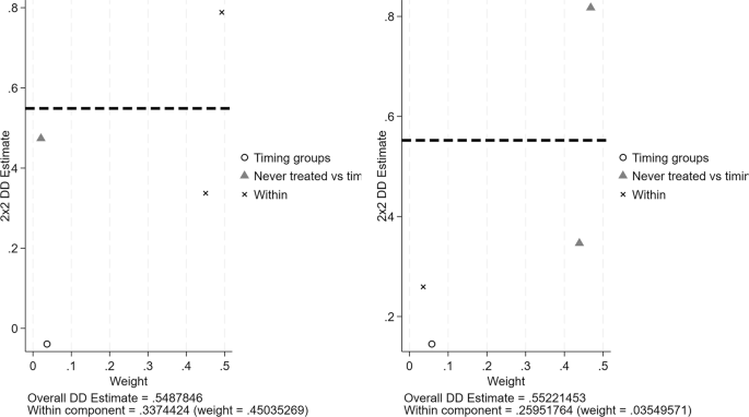
Bacon decomposition diagram (the graph on the left has covariates, and the graph on the right has no covariates).
As seen from the decomposition results in Fig. 5 and Table 6, the forbidden control group (represented by a circle) has a small weight and does not affect the estimated results of the baseline regression, regardless of whether there are covariates. The results of Bacon decomposition once again prove the robustness of the benchmark regression results.
An important potential problem of staggered DID is the existence of heterogeneous processing effects; that is, the same processing has different effects on different individuals. The TWFE estimator is a weighted average of the “good” comparison and the “bad” comparison in the presence of heterogeneous effects, and it breaks the parallel trend hypothesis, so the obtained estimator may have bias. Reference of this research. In the method proposed by Callaway and Sant ‘Anna (2021), aipw estimators are used for testing. The results are shown in Fig. 6.

Each individual can be divided into several groups according to the different times when they are affected by the policy. The upper left of Fig. 6 shows the test results of different individuals at the time points of two policy shocks. Before the second policy shock, the 95% confidence interval includes 0, and after the policy shock, the 95% interval does not include 0, passing the parallel trend test. The upper right part of Fig. 6 shows the test of the average treatment effect of the treatment group. The figure shows that the value of ATET decreases first and then increases when the contact treatment time increases. This may indicate that the effect of treatment varies over time and that there may be an adaptation period or delayed effect. This result also mirrors the parallel trend test of the benchmark regression model, which shows no significant positive effect in the first two years after the implementation of the policy.
Path of ecological sustainability policy affecting rural income
In this section, this study explores the path mechanism through which ecological sustainability policy affect rural income. In the process of implementing the national key ecological function zone policy, agricultural revitalization, industrial support, and ecological value transformation are the core measures used to promote rural income. Therefore, this study examines these three paths. Tables 7–9 list the estimated results.
Table 7 presents the test results for agricultural revitalization, indicating that the ecological function zone policy can increase rural residents’ income by promoting agricultural revitalization. The results in the first and second columns of Table 7 show that the national key ecological function zone policy increased crop planting area and grain production by 108% and 8.4%, respectively, and these effects were statistically significant at the 1% level. The results in Tables 3 and 4 show that agricultural value added and agricultural labor productivity increased by 6.6% and 6%, respectively. The results in Table 7 show that the ecological functional zone policy significantly increased oilseed crop production by 19%. Planting high-yield oilseed crops is an important driver of agricultural revitalization. The results in the sixth column show that agricultural mechanization levels increased significantly by 19%, indicating that promoting agricultural mechanization in ecological functional zones is an important pathway to enhance local agricultural output. Agricultural output is the primary source of farmers’ income. Agricultural revitalization can increase agricultural output, playing a key role in reducing the urban-rural income gap (Tan et al., 2025b) and holding significant implications for the poor (Christiaensen et al., 2011). It is a critical driver of rural income development, thus validating Hypothesis H2a.
The possible reasons are as follows: the implementation of key ecological functional zone policies can improve organic carbon storage in different functional zones (Gao et al., 2024), improve local soil quality, and promote relevant indicators of agricultural revitalization, such as the sown area of crops and grain output. An increase in the acreage of crops may increase the yield of food at harvest. An increase in grain production helps improve the competitiveness of farmers in the agricultural market, increases the sales of grain, and promotes the improvement of farmers’ income. The improvement in agricultural labor productivity and agricultural machinery power means that more agricultural products can be produced per unit time, reducing labor costs and increasing rural residents’ income.
Table 8 presents the results of the industrial support analysis. The findings indicate that China’s key national ecological function zones can increase rural residents’ income by promoting industrial support. As shown in the first and second columns of Table 11, compared with non-national ecological function zones, the entrepreneurial activity in the primary sector within national key ecological function zones increased by 9.1% at the 1% significance level. The estimated results in the second column also show that ecological function zone policies significantly promote the development of forestry, animal husbandry, and fisheries. Additionally, this paper further examines how these effects contribute to income growth among residents. According to the estimated results in the third and fourth columns, the number of employed individuals in the secondary and tertiary industries within ecological function zones increased by 11.2% and 7.3%, respectively, compared to non-ecological function zones. These results indicate that the policy has promoted entrepreneurial activity in the primary sector and employment in the secondary and tertiary sectors, achieving industrial support and revitalization, narrowing the urban-rural income gap (Chen et al., 2025), and further promoting income growth in rural areas. Therefore, hypothesis H2b is validated.
The possible reasons are as follows: First, the implementation of the ecological functional zone policy has improved local air quality, soil conservation, and biodiversity, attracting many enterprises to invest in the construction of rural areas and increasing employment opportunities for local residents. The increase in enterprises not only provides a stable source of income for local residents but also improves the quality and employability of the rural labor force through skill training and technology transfer (Jin et al., 2010). Second, the development of secondary and tertiary industries, especially tourism services, attracts tourists, promotes consumption and increases the income of local residents by making full use of local natural and cultural resources. Industrial development also contributes to the formation of an industrial chain, drives the development of related industries such as forestry, and promotes industrial integration, thus increasing the income of rural residents once again (Wang et al., 2024a).
Table 9 shows the results of the ecological value conversion test. The results indicate that ecological value conversion is one of the key mechanisms for enhancing rural residents’ income in national key ecological functional zones. As shown in the first and second columns of Table 9, after the implementation of the national key ecological functional zone policy, carbon emissions decreased significantly by 3.7%, and the Normalized Difference Vegetation Index (NDVI) increased significantly by 6.2%. The estimated results in the third column also show that the value of ecosystem services has significantly increased by 1.6% after the implementation of the ecological functional zone policy. Additionally, this study further examined the impact of the ecological functional zone policy on ecological efficiency, specifically the CEIP. According to the estimated results in Table 4, the CEIP in ecological functional zones decreased by 11% compared to non-ecological functional zones, indicating that the implementation of the ecological functional zone policy can effectively alleviate the carbon carrying capacity per unit of green space. These results indicate that the ecological functional zone pilot policy promotes the conversion of ecological value, improves the quality of life for local residents, and enhances residents’ environmental income (Angelsen et al., 2014), thereby increasing rural income. Therefore, hypothesis H2c is validated.
The implementation of an ecological function zone policy improves the local ecosystem, reduces carbon emissions, and reduces the risk of abnormal weather, which in turn promotes the narrowing of economic differences between regions (Dell et al., 2012) and narrowing the income gap. As the ecosystem is improved, the ecological value it creates is further transformed. The improvement and transformation of the NDVI promote the growth of local crops so that the output of agricultural products may increase, improve the competitiveness of local residents in the agricultural market, and improve income levels. In addition, the implementation of an ecological functional zone policy can improve residents’ environmental income and quality of life by increasing the value of ecosystem services and the green coverage rate (Angelsen et al., 2014).
Heterogeneity analysis
Considering that different ecological functions have different functional characteristics, such as water conservation, wind prevention and sand fixation, there may be differences in policies. Besides, different ecological functional areas have different effects on plant growth because of their different functions, and the income of residents may also be affected. Hence, this study divided the NDVI of different counties and the redisents’ income of different ecological functional areas to analyze the heterogeneity of the policy effects of key national ecological functional areas. The specific estimation results are shown in Table 10.
The estimated results in Table 10 show that in areas with lower NDVIs and income levels, the national key ecological functional zone policies have a more significant effect on income promotion. Specifically, Columns 1 and 2 in Table 10 show the heterogeneity test results for different NDVIs. The regression coefficient of DID in column 1 was 0.482 and was significantly positive at the 1% level, whereas the coefficient of DID in column 2 was positive but not significant, indicating that the policy effect of ecological functional areas was more obvious in regions with lower NDVIs. Columns 3 and 4 show the heterogeneity test results for different income levels. The coefficients of column 3 DID are positive and significant at the 1% level, whereas the coefficients of column 4 DID are positive and significant at the 5% level. After the regression of samples is performed, the direct comparison coefficient size will produce bias. In this study, the Chow test and Fisher combination test were performed on the grouping regression results of columns 3 and 4 with reference to the test method proposed by Chow (Chow, 1960). The test results, combined with the regression coefficients of Columns 3 and 4, show that in areas with lower income, ecological functional zones have more obvious promoting effects on policies.
Different regions have distinct initial resource endowment characteristics, and policy outcomes may vary accordingly. For instance, local governments may select specific poverty alleviation measures based on their comparative advantages. Consequently, in regions with better initial development conditions, implementing poverty alleviation policies may lead to faster growth in local industrial and agricultural output (Li et al., 2024c). National key ecological functional zones consist of a series of different types of functional zones, and the initial natural resource endowment characteristics of these different functional zones also vary. Therefore, not only may policy effects differ, but the pathways through which different functional zone types influence rural income may also vary. Due to space constraints, the data processing methods, regression results, and interpretations are included in the Appendix C, and readers may refer to them directly.
Further discussion based on the stratified analysis method
In randomized controlled trials, randomization ensures that the characteristics of study subjects are balanced between the experimental group and the control group. The experimental group and control group for policy variables are typically determined by a national government, resulting in non-randomized outcomes. If grouping is unbalanced, it can lead to confounding bias, and controlling for covariates is an important consideration in statistical analysis. Given that the policy variable in this study is a binary categorical variable, the study employs stratified analysis to divide multiple important factors into subgroups and conduct independent analyses within each subgroup, thereby mitigating confounding bias. This study discretised the dependent variable (rural income) and continuous covariates based on their quantiles. The variables of economic development, science and technology, and public expenditure were selected as the representative stratification variables for regional income characteristics. The results are shown in Tables 11–13.
The second column in Tables 11–13 represents the DID binary classification variable, while the third and fourth columns show the classification results and their respective proportions within each stratum. For example, the third column in Table 11, “7375” indicates that there were 7375 cases in the low-income group in regions with low economic development and no pilot policies between 2007 and 2022, accounting for 90.2% of the low-income population. The fifth column shows the OR (Odds Ratio) values, indicating the relative strength of the treatment across different strata, with the lower and upper confidence limits in parentheses. The sixth and seventh columns show the chi-square value and the p-value of the test, respectively. The results in Table 11 indicate that there is a statistically significant association between the national key ecological function zone policy and income levels in both the low economic development and high economic development layers. This association persists even when economic development is not considered. The results of the Mantel-Haenszel generalized ratio estimate test indicate that the confounding bias of economic development underestimates the true association between policy and income. The results in Table 12 indicate that there is a statistically significant association between national key ecological function zone policies and income levels in both the low technology and high technology strata, and this association persists even when the innovation factor is excluded. The results of the Mantel-Haensel generalized ratio estimate test indicate that the confounding bias of technological innovation underestimates the true relationship between policy and income. The results Table 13 indicate that the confounding bias of public expenditure overestimates the true relationship between policy and income.
Decision-making framework based on the research results
Sections 4.1 to 4.10 present the empirical findings of this study in detail. Prior to formulating systematic policy recommendations, this research proposes a decision-making framework based on empirical evidence to enhance the operability of strategies, thereby directly demonstrating the practical value of the research outcomes, as illustrated in Fig. 7. Figure 7 presents the decision-making framework derived from the research findings. First, given that the national pilot policy for key ecological function zones aims to increase rural residents’ income through agricultural revitalization, it introduces digital management platforms, conducts labor skills training, and implements green transformation of traditional agriculture via industrial ecologization. Incorporating agricultural labor productivity and green technology adoption rates into local government performance evaluations creates policy-driven momentum. Second, leveraging the policy’s characteristic of boosting rural income through industrial support, systematically deploy industrial chains such as agricultural processing (ecological agriculture), eco-tourism, and rural entrepreneurship within functional zones. Strengthen investment guidance to promote diversified development of ecological agriculture, eco-tourism, and related industries. Third, capitalizing on the policy’s feature of increasing rural income through ecological compensation, the core lies in linking compensation amounts to ecological benefits and ecosystem service values while implementing performance incentive mechanisms. And leverage green and low-carbon technologies to expand the scale and realize the value of ecological industries through industrialization pathways. Fourth, recognizing that ecological functional zone policies effectively boost rural incomes in areas with lower resource endowments and underdevelopment, implement differentiated policies tailored to local conditions. Provide targeted support to regions with fragile ecosystems and low incomes—such as increased fiscal investment and compensation, ecological technology training, and infrastructure support—to ensure precise policy implementation.
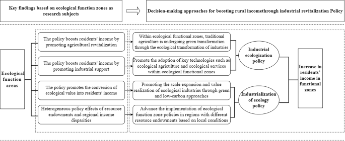
Decision-making framework based on the research results.
link